Friday, November 16, 2018

Differential Pressure Transmitters (DP)

One of the most common and useful pressure measuring instrument used in most industrial measurement applications is the differential Pressure transmitter. This device senses the difference in pressure between two ports and outputs a signal representing that pressure in relation to a calibrated range.
Differential Pressure transmitters constructed for industrial measurement applications typically consists of a strong (forged metal) body housing the sensing element(s), topped by a compartment housing the mechanical and/or electronic components necessary to translate the sensed pressure to a standard instrumentation signal e.g. 3-15 PSI, 4-20 mA, Digital Fieldbus codes as shown in the below Diagrams:
Differential Pressure Transmitters

In the below example of Rosemount differential pressure transmitter, the pressure-sensing element is housed in the bottom half of the device (forged-steel structure) while the electronics are housed in the top half (the coloured, round, cast-aluminium structure)
Differential Pressure Transmitter

Every differential Pressure (DP, d/p or ∆P) transmitter has two pressure ports to sense different process fluid pressures. These ports typically have ¼ inch female NPT threads to readily accept connections to the process. One of these ports is labelled “high” and the other is labelled “low’’. This labeling does not necessarily mean that the “high” port must always be at a greater pressure than the “low’’ port. What these labels represent is the effect any increasing fluid Pressure applied to that port will have on the direction of the output signal’s change. Note that, a differential pressure instrument responds only to differential pressure while ignoring the common-mode pressure (gauge pressure common to both ports).
Differential Pressure Transmitters Low and High Ports

The most common sensing element used by modern DP transmitters is the diaphragm. One side of this diaphragm receives process fluid pressure from the “high’’ port while the other receives process fluid pressure from the “low’’ port. Any difference of pressure between the two ports causes the diaphragm to flex from its normal resting (center) position. This flexing is then translated into an output signal by any number of different technologies depending on the manufacturer and the transmitter model.
Differential Pressure (DP) Transmitter Applications
The combination of two differential pressure ports makes the DP transmitter very versatile as a pressure-measuring device. This one instrument can be used to measure pressure differences, positive (gauge) pressures, negative (vacuum), and even absolute pressures, just by connecting the “high” and “low” sensing ports differently.
In every DP transmitter application, there must be some means of connecting the transmitter’s pressure-sensing ports to the points in a process. Metal or plastic tubes (or pipes) work well for this purpose, and are commonly called impulse lines or gauge lines or sensing lines. Typically these tubes are connected to the transmitter and to the process by means of compression fittings which allow for relatively easy disconnection and re-connection of tubes.
Key applications of DP transmitters include:
Measuring Process Vessel Clogging – We may use the DP transmitter to measure an actual difference pressure across a process vessel such as a filter, a heat exchanger, or a chemical reactor. The diagram below shows the use of a DP transmitter to measure clogging of a water filter:
Differential Pressure Transmitter Industrial Applications

From the diagram above, you can see the high side of the DP transmitter connects to the upstream side of the filter and the low side of the transmitter to the down side of the filter. This way, increased filter clogging will result in an increased transmitter output. Since the transmitter’s internal pressure-sensing diaphragm only responds to differences in pressure between “high” and “low” ports, the pressure in the filter and pipe relative to the atmosphere is completely irrelevant to the transmitter’s output signal. The filter could be operating at a line pressure of 15 PSI or 15000 PSI – the only variable the DP transmitter measures is the pressure drop across the filter. If the upstream side is 15 PSI and the downstream side is 14 PSI, the differential pressure will be 1 PSI sometimes labelled PSID, where “D” is differential. If the upstream pressure is 15000 PSI and the downstream pressure is 14,999 PSI, the DP transmitter will still see a differential pressure of just 1 PSID.
Measuring positive gauge pressure – DP instruments can also serve as gauge pressure instruments. If we simply connect the “high” side of a DP instrument to a process vessel using an impulse tube, while leaving the “low” side vented to atmosphere, the instrument will interpret any positive pressure in the vessel as a positive difference between the vessel and the atmosphere. 
Differential Pressure Transmitter Industrial Applications

Most DP instrument manufacturers offer gauge pressure versions of their differential instruments with “high” side port open for connection to an impulse line and the “low’’ side of the sensing element capped off with a special vented flange, effectively performing the same function as in the above figure.
Measuring absolute Pressure – Absolute pressure is defined as the difference between a given fluid pressure and a perfect vacuum. We may build an absolute pressure sensing instrument by taking a DP transmitter and sealing the “low” side of its pressure-sensing element in connection to a vacuum chamber as shown below. This way, any pressure greater than a perfect vacuum will register as a positive difference.
Differential Pressure Transmitter Industrial Applications

Measuring Vacuum – The same principle of connecting one port of a DP device to a process and venting the other works as well as a means of measuring vacuum (Pressure below that of atmosphere). All we need to do is connect the “low” side to the vacuum process and vent the ‘’high” side to the atmosphere as shown below: 
Differential Pressure Transmitter Industrial Applications

Any pressure in the process less than atmospheric will register to the DP transmitter as a positive difference (with P-high   greater than P-Low ). Thus the stronger the vacuum in the process vessel, the greater the signal output by the transmitter.
Inferring liquid level – Liquids generate pressure proportional to height (depth) due to their weight. The pressure generated by a vertical column of liquid is proportional to the column height (h), and liquid’s mass density (ρ), and the acceleration of gravity (ɡ):        P=ρɡh
Differential Pressure Transmitter Industrial Applications

As the liquid in the vessel increases, the amount of hydrostatic pressure applied to the transmitter’s ‘’high’’ port increases in direct proportion. The width of the vessel is irrelevant to the amount of pressure produced only the liquid height (h), density (ρ), and gravity (ɡ) are significant. Thus the transmitters increasing signal represents the height of liquid inside the vessel no matter the size or shape of the vessel.
h = P/ρɡ   
Inferring gas and Liquid Flow – DP transmitters are widely used in measurement of fluid flow. Pressure dropped across a constriction in the pipe varies in relation to flow rate (Q) and fluid density (ρ). So long as fluid density remains fairly constant, we may measure pressure drop across a piping constriction and use that measurement to infer flow rate. The most common form of constriction is the orifice plate. This is a metal plate with a precisely machined hole in the center. As fluid passes this hole, its velocity changes, causing a pressure drop to form.
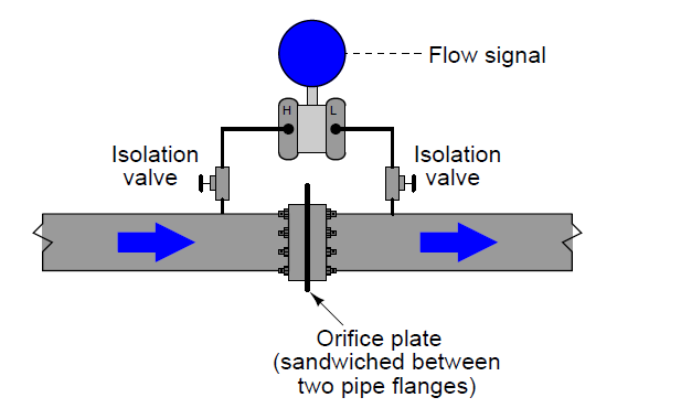
Differential Pressure Transmitter Industrial Applications

Since both ports of the transmitter connect to the same process line, static fluid pressure within that line has no effect on the measurement. Only differences of pressure between the upstream and downstream sides of the constriction (orifice plate) cause the transmitter to register flow.
Don't miss out on key updates, join our newsletter list here.

Tuesday, November 6, 2018

How to Wire a 4-20 mA Current Loop

A 4-20 mA current loop is a series of connected elements like flashlight batteries. The elements of a current loop are connected in series. An easy way to remember the connections is (+)  (-), (-)  (+), then reverse the power supply connections (+) (+), (-) (-).
Wiring a 4-20 mA current loop

When we redraw the above circuit, we get to know how to wire into a junction box as shown below:
Wiring a 4-20 mA current loop

To add a PLC or computer input, we just insert into the loop. Always remember the (+)  (-), (-)(+) except at the power supply.
Adding a computer or PLC input, the wiring will look as follows:
Wiring a 4-20 mA current loop

Please note that you can only make one ground in a 4-20 mA system. Multiple grounds will cause erroneous readings.
Important items that must be checked when determining loop compliance or Power supply voltage:
  • The compliance voltage must be great enough to fully power all the loop devices at 20 mA. It is usually better to assume 25 mA max to allow yourself some ''head room''. You must also have enough voltage available to account for the drop in the wires. 
  • The loop power supply voltage must not exceed the maximum voltage rating of any device in the loop e.g. the transmitter above the maximum loop voltage of 30 VDC. Be aware of safety. If you are using low voltage wiring, you generally want to keep the voltage below 28 VDC. 
  • Note that, to calculate the required loop power supply (for compliance purpose), you add  up the voltage drops around the loop at the highest expected current. Loop powered devices (like the transmitter and meter above), will tell you the required voltage in their data sheets. 
Don't miss out on key updates, join our newsletter list here.

How Pitot Tubes are used in Flow Measurement

Pitot tube sensors, orifice plates, flow nozzle or venturi tubes are classified as flow measuring devices which utilize differential pressure to measure volumetric flow. 

Pitot Tube Sensor

The Measuring Principle of Pitot Tube
The measuring principle of the pitot tube utilizes the differences between the pressure ridge on the upstream side of a bluff body and the static pressure on its down stream side.
Pitot Tube Measuring Principle

We have differences in pressures at S2 and S1. This difference in pressures is measured, then converted into fluid flow velocity, from this we can derive the volumetric flow using the continuity law with a pipe area A and an average flow velocity. i.e. Q=VA where Q is the volumetric flow, V is the average velocity and A is the pipe area.
Required fluid conditions 
To have good measurements from pitot tube sensors, we need to satisfy the following conditions:
  • The fluid has to completely fill the pipe so that the measured differential Pressure is representative of the volumetric flow. Fluids in partially filled pipes can only be measured if a full pipe can be arranged e.g. by means of siphon. 
  • The fluid must be single-phase. Two phase fluids e.g. water-air mixtures cannot be measured. 
  • The flow has to be sufficiently turbulent. Fluids of laminar nature cannot be measured with pitot tubes.
  • Fluid may contain small particles or bubbles. The pressure generated in front of the sensor apertures causes a deflection of the particles or bubbles. Fluids which tend to crystallize will quickly plug the pressure tubes of the sensor and therefore cannot be measured with pitot tubes. 
  • In steam measurement applications condensate pots are used inside of which a constant transition from steam to condensate and vice versa occurs. The pressure transfer is achieved via water columns. 

Industrial Applications of Pitot Tube Flowmeters
Pitot tube sensors are mainly used to measure the volumetric flow of liquids, gases and steam in closed pipes ranging from½“ to 480“ (DN 20 to DN 12000).
Examples of specific applications include: Precise volumetric flow measurement in batch processes, continuous measurement of liquid ingredients in the process industry, fuel, air, steam and gases as primary energy source as well as in control functions requiring a high degree of stability and repeatability.
Advantages of pitot tubes over orifice plates
  • They have a lower permanent pressure loss as compared to orifice plates. 
  • They have a shorter up/down straight pipe run requirements as compared to orifice plates. 
  • The profile of Pitot tube sensors is designed such that it is symmetrical to the plane between the pressure channels. This arrangement results in the same resistance values and thus the same k-factor with respect to the fluid properties during forward as well as reverse flow. The differential pressures generated by a given flow velocity are the same for flow in either direction. The only differ in the +/- sign. This constitutes an advantage of the orifice plate. Consider the figure below, of an orifice plate which because of its angled downstream corner has different resistances values for forward and reverse flows. It would indicate widely different pressures for the same flow velocity in opposite directions.
Orifice Plate Flow measurement


Some of the manufacturers of Pitot tube flow measurement Instruments, include:

Don't miss out on key updates, join our newsletter list here.

Monday, November 5, 2018

The Working of Distributed Control Systems

Distributed control system (DCS) is a computerized control system used to control production line in most industries.

Importance of DCS systems
In most cases, products go through many stages in the factory before they reach their final stage. During their passage through those stages, it requires a kind of control in order to adjust the quality of the each product. To adjust quality, you need to control many physical quantities such as Pressure, Temperature, Level, Flow etc. In petrochemical factories and nuclear reactors the control of these parameters is very critical, in fact losing control may lead to an explosion of the whole plant.
So what are the key components that make up a DCS system?
A DCS system consists of:
Programmable Logic Controllers (PLC): These includes input or output modules, CPU, Communication bus, interface module, PS etc.
Operator Station: It is basically human interface machine (HMI) with a monitor, the operator man can view the process in the plant and check if an alarm is present, change any setting, or print reports etc.
Engineering Station: It is used to configure all input & output module, make drawing of anything required and also, monitors an operator station.
The following diagram shows  a Basic Block Diagram of a DCS system:
Block Diagram of a DCS system

The Working of a DCS system
The DCS system receives input signals from other devices, these signals will be processed and analysed by the CPU and based on the result, an action will be taken. There are many sensors and transducers inside the plant which converts physical quantities such as temperature, pressure, level, flow to an electrical quantity and also transmits the electrical signals representation to the DCS system.
The electrical signals could either be analog or digital signals, they could be in either of the two forms: 4-20 mA or 1-5 VDC
The digital signals could either be logic 0 or logic 1
When the PLC receives the analog signals from different transmitters it will convert it to digital signals via input module then pass it to the CPU for processing. The CPU will compare the process measured value (PV) with the set point value (SV). If both the values are not matched, then the DCS will generate an output called manipulated value (MV) to the field via output modules in order to adjust the physical quantity by for example controlling the opening or closing of a valve.
On the face plate, the operator can see both parameters reading SV and PV. The SV can be set to the required level by the operator. DCS system will operate the pump by sending MV signal via output module to fill the tank and continue as long as PV signal received from the transmitter is less than the SV. Once the water level reaches the required point i.e. PV=SV, the DCS will stop the pump and this happen if face-plate mode is AUTO, however in MANUAL mode, the operator can control MV directly and SV pointer will be disabled. This is a simple working of a DCS system. You may find different physical quantities being controlled, it could be the flow rate or pressure in the system.
Some of the leading manufacturers of DCS systems include:

Don't miss out on key updates, join our newsletter list here.

Wednesday, October 24, 2018

Instrumentation and Control Symbols

Here we look at common instrument symbols used in various types of technical diagrams that are used to document instrument systems.

Instrument Bubbles
Instrument Bubbles

Line Types
Instrumentation Line types Symbols

Note that, the single backlash signifying discrete or binary type has been removed from ISA standard. Regular Pneumatic and Electrical Line Symbols may represent either continuous or discrete states. 

Process/Instrument Line Connections
Process/Instrument line connections


Process Valve Types
Process Valve Types


Valve Actuator Types

Valve Failure Mode
Valve Failure Mode
Liquid Level Measurement Devices
Liquid level measurement devices

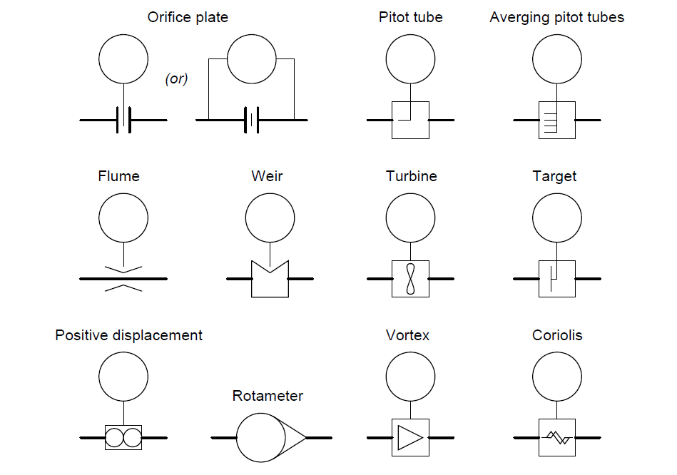
Flow Measurement Devices  (Flowing from left to right)
Flow Measurement devices
Flow Measurement Devices

Process Equipment Symbols

Functional Diagrams Symbols
Functional Diagrams symbols

Single-line electrical diagram
single line electrical diagrams
Single-line electrical diagram

Fluid Power Diagram Symbols
You can also read: 

Don't miss out on key updates, join our newsletter list here.

Tuesday, October 23, 2018

Functional Diagrams

Functional Diagrams form part of diagrams used In Instrumentation. In our previous articles, we looked at Process Flow Diagrams, Process & Instrument Diagrams as well as Loop Diagrams.
In this article, we look at a unique form of technical diagram for describing functions comprising a control system (e.g. PID Controllers, Rate Limiters, Manual Loaders). The diagrams used to document control strategies are termed as functional diagrams. Note that, functional diagrams focus on the flow of information within a control system rather than on the process piping or instrument interconnections i.e. wires, tubes etc. The general flow of a functional diagram is top-to-bottom, with the process sensing instrument (transmitter) located at the top and the final control element (valve or variable-speed motor) located at the bottom.
Functional  Diagrams are all about the algorithms used to control decisions, so no attempt is made to have the symbols arranged to  correspond with actual equipment layout. 
Let's consider a functional diagram shown below:
Functional Diagrams

The above functional diagram shows a flow transmitter (FT) sending a process variable signal to a PID Controller, which then sends a manipulated variable to a flow control valve (FCV).
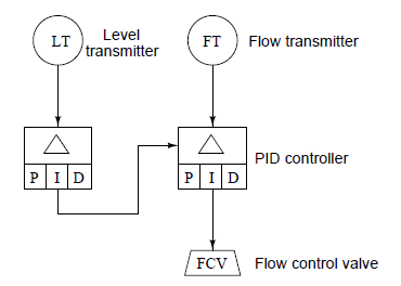
A cascaded control system, where the output of one controller acts as the set-point for another controller to follow, appears in functional diagram as shown below:
Functional Diagram


In the above cascaded control system, the primary controller senses the level in a vessel, commanding the secondary (flow) controller to maintain the necessary amount of flow either in or out of the vessel as needed to maintain level at some point.
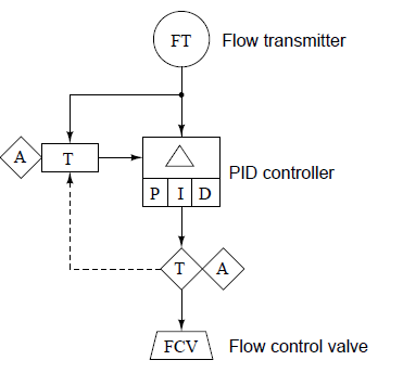
Functional diagrams may show varying degrees of detail about the control strategies they document e.g. you may see the auto/manual controls represented as separate entities in a functional diagram, apart from the basic PID controller function. In the following Functional Diagram, a transfer block (T) and two manual adjustment blocks (A) providing a human operator with the ability to separately adjust the controller’s set point and output (manipulated variables) and to transfer between automatic and manual modes:
Functional Diagrams

Rectangular blocks such as the Δ, P, I and D shown in the diagram below represent automatic functions.  Diamond-shaped blocks such as A and T blocks represent manual functions which must be set by a human operator. The Functional diagram also shows the presence of set point tracking in the controller algorithm, a feature that forces the set point value to equal the process variable value any time the controller is in manual mode.
Functional Diagrams

A solid line in a functional diagram represent analog (continuously variable) signals such as process variable, set point, and manipulated variable. Dashed lines represent discrete (on/off) signal paths, in this case the auto/manual state of the controller commanding the PID algorithms to get its set point either from the operator’s input (A) or from the process variable input (the flow transmitter: FT).
Don't miss out on key updates, join our newsletter list here.

Monday, October 22, 2018

Loop Diagrams


Having looked at the PFD and P & ID Diagrams in our previous posts, we can now discuss the loop diagrams also called the loop sheets. Let's consider the diagram of a compressor surge system shown below:
Loop Diagram
From the loop diagram above we can see more additional instruments that weren’t shown in the PFD and  P & ID: We have 2 transmitters, a controller, and a valve. We also have 2 signal transducers. The first transducer  42a modifies the flow transmitter signal before it goes into the controller. and the second transducer 42b converts the electronic 4-20mA signal into a pneumatic 3-15 PSI air pressure signal. Each instrument  ''bubble''  in a loop diagram represents an individual device, with its own terminals for connecting wires.
The dashed lines represent individual copper wires instead of whole cables. Terminal blocks where these wires connect to are represented by squares with numbers in them. Cable numbers, wire colors, junction block numbers, panel identification and even grounding points are all shown in the loop diagrams.  You can also notice from this loop diagram, the action on each instrument. You will see a box and arrow (pointing either up or down) next to each instrument bubble. An ” up” arrow () represents a direct-acting instrument: one whose output signal increases as the input stimulus increases. A down arrow () represents a reverse-acting instrument, one whose output signal decreases as the input stimulus increases.
All the instruments in this loop are direct-acting with the exception of the pressure differential transmitter PDT-42. Here the down arrow tell us that the transmitter will output a full-range signal (20 mA) when it senses zero differential pressure, and a 0% signal (4 mA) when it sensing a full 200 PSI differential. Excessive pressure drop across the compressor is considered dangerous because it may lead to the compressor surging. For this reason, the controller will naturally take action to prevent surge by commanding the anti-surge control valve to open, because it, “thinks” the compressor is about to surge i.e. the transmitter is intentionally calibrated to be reverse-acting such that any break in the signal wiring will naturally bring the system to its safest condition.
The only diagram that can be more detailed than a loop diagram is the electronic schematic diagram for an individual instrument but then it shows details for that particular instrument alone, thus the loop diagram is the most detailed form of diagram for any control system as a whole and it must contain details omitted by PFDs and P & IDs.            

Sunday, October 21, 2018

Process and Instrument Diagrams (P & IDs)


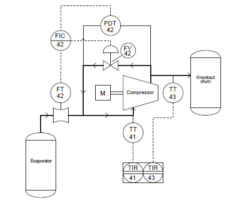
In the previous post, we looked at Process Flow Diagrams (PFDs),  where we indicated that a PFD represents a big picture of the entire process. In this post, we look at the Process and Instrument Diagrams (P & IDs), where we will try to get more details that weren’t shown in the PFD. Let's consider the compressor control system diagram below:
Process and Instrument Diagrams ( P & IDs)

From the above, we can see that there is more instrumentation associated with the compressor than just a flow transmitter. We have the differential pressure transmitter (PDT), a flow indicating controller (FIC), and a recycle control valve (FV42), that allows some of the vapor coming out of the compressor discharge line to go back around the compressor suction line. Also, we have a pair of temperature transmitters (TT41 & TT43) reporting suction and discharge line temperatures to an indicating recorder.
Additional details emerge in the P & ID above, the flow transmitter, flow controller, pressure transmitter and flow valve all bear a common number 42. This common, ”loop number” indicates these four instruments are all part of the same control system. An instrument with any other loop number is part of a different control system, measuring and/or controlling some other function in the process like the two temperature transmitters and their respective recorders, bearing the loop numbers 41 and 43.
You can also read: Process Flow Diagrams
The other information we can derive from the P & ID above, are the different instrument ” bubbles” used. Some of the bubbles are just open circles, while others have lines going through the middle as shown below:
Process and Instrument Diagrams

Process and Instrument Diagrams

Each of these symbols have meaning according to the ISA ( Instrumentation, Systems and Automation Society).
The type of “bubble” used for each instrument tells us something about its location. The rectangular box enclosing box enclosing the temperature recorders (TIR 41 and TIR 43) shows they are part of the same physical instrument i.e. this indicates that there is really only one temperature recorder instrument, and that it plots both suction and discharge temperatures (most likely on the same trend graph). This suggests that each bubble may not necessarily represent a discrete, physical instrument, but rather an instrument function that may reside in a multi-functional device.
The P & ID shows more details than PFD, but we cannot see other details like the cable types, wire numbers, terminal blocks, junction boxes, instrument calibration ranges, failure modes, power sources etc. To examine this level of details, we need to look at the loop diagram.
Don't miss out on key updates, join our newsletter list here.